15 Columns
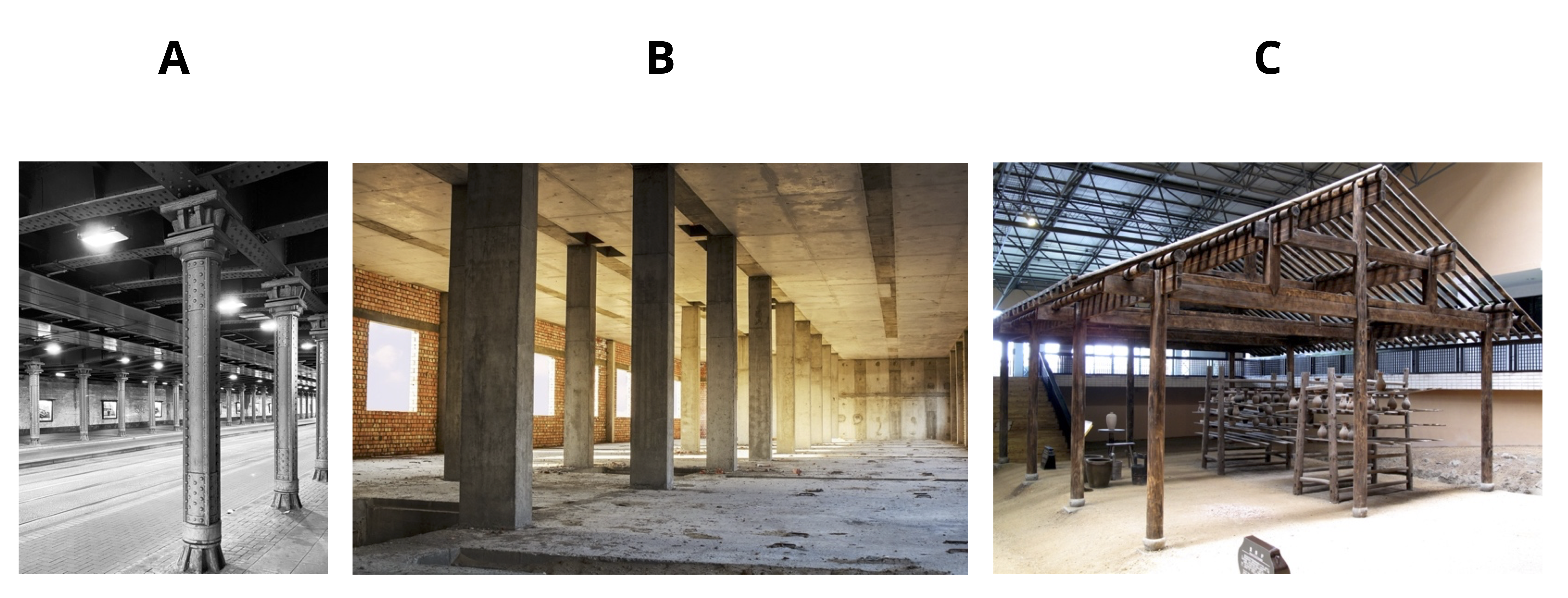
Until now our focus has been primarily on meeting strength and deflection criteria. While these aspects are crucial, it’s equally important to ensure a structure’s stability. This chapter therefore delves into the stability analysis of long and slender members subjected to compressive loading, commonly referred to as columns. Some examples are shown in Figure 15.1. When the compressive load reaches a critical point, columns may undergo sudden sideways deflection, a phenomenon known as buckling. After buckling, a column is unable to support any further load. This chapter focuses on long, slender, homogeneous, axial compression members, otherwise known as columns.
Section 15.1 derives the buckling formula for columns that are supported by pin connections at both ends. Section 15.2 extends this to consider other common end conditions.
15.1 Euler’s Formula for Buckling
Click to expand
Even in ideal conditions, buckling often occurs for long, slender members at loads significantly lower than the material’s crushing or compression limit. When a long, slender object is subjected to axial loading, it may buckle once the load reaches a critical threshold known as the critical load, Pcr. At this point the object experiences significant lateral deflection perpendicular to the load direction, so columns should be designed such that the applied load does not exceed the critical load.
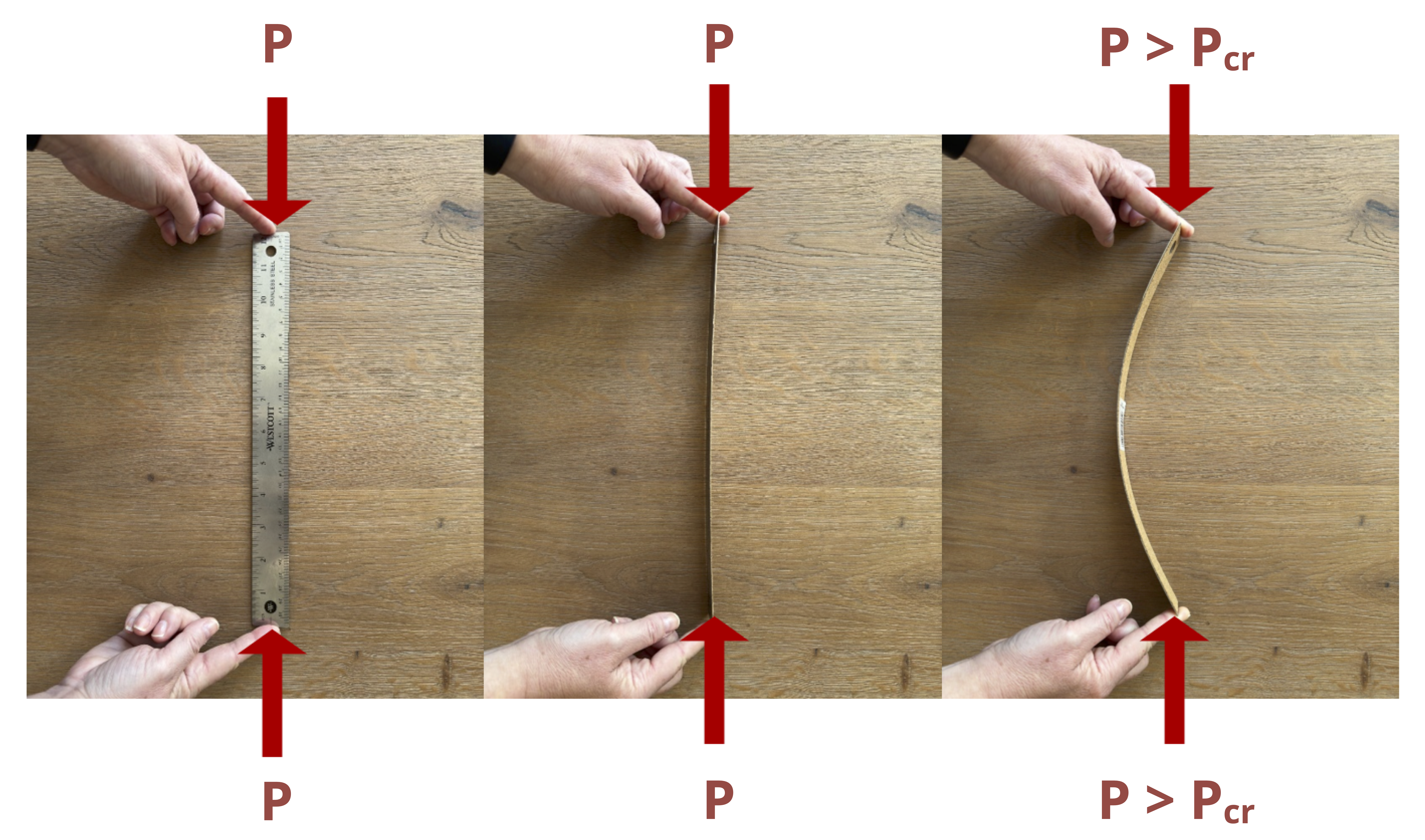
Buckling of a ruler (long, slender member) is depicted in Figure 15.2. The ruler in the left and center photos is subjected to axial load, P, that is less than critical load, Pcr. This is known as stable equilibrium. In the photo on the right the axial load P exceeded the critical load Pcr, causing a significant lateral deflection. This is known as unstable equilibrium.
15.1.1 Stability
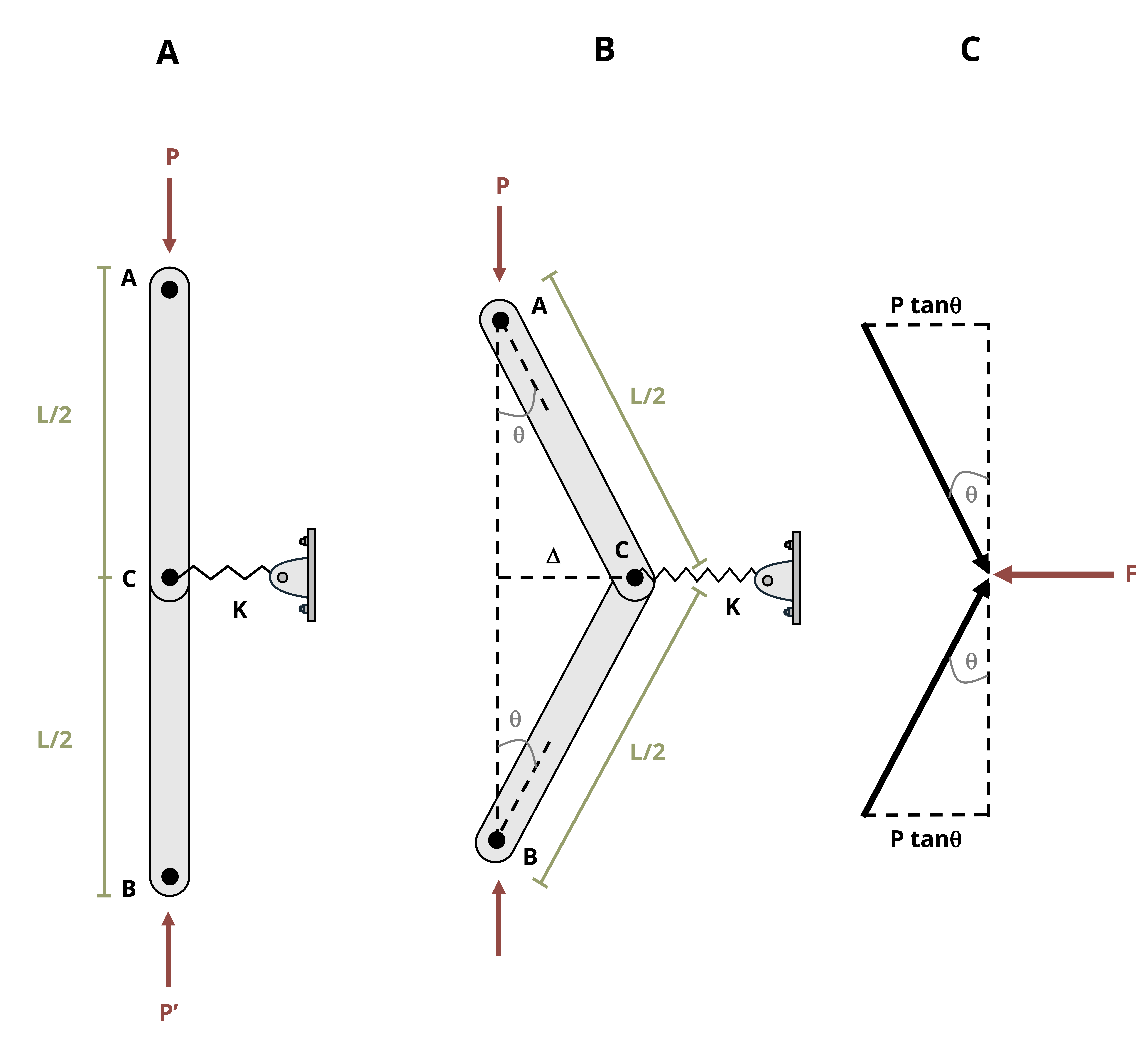
We can consider stability by using a simplified model of a pinned-pinned column. This column consists of two ridged bars connected with a pin and a spring with a stiffness k, as the free body diagram (FBD) shows in Figure 15.3 (A). When the load, P, is small, the system remains vertical and the spring is unstretched. If point C is displaced to the right a small amount, Δ, the spring will produce a force F = kΔ, as shown in Figure 15.3 (B). This force is used to resist the horizontal forces, Px = Ptanθ, as shown in Figure 15.3 (C).
Since θ is small
\[ \sin \theta \sim \theta \text { and } \tan \theta \sim \theta \]
Consequently
\[ \Delta=\theta \frac{L}{2} \text { and } 2 P_x=2 P \theta \]
Using the spring restoring force equation F = kΔ, then substituting in for Δ, results in
\[ F=k \theta \frac{L}{2} \]
If the spring restoring force is greater than the axial force, then equilibrium is stable.
\[ \begin{aligned} & F>P \\ & k \theta \frac{L}{2}>2 P \theta \end{aligned} \]
The θ cancels out, and we can solve for P.
\[ P<\frac{k L}{4} \]
Similarly, we can solve for the expression for unstable equilibrium F < P.
\[ P>\frac{k L}{4} \]
The point at which F = P is crucial because it is the line between stable and unstable equilibrium. This is known as the critical load Pcr.
\[ P_{c r}=\frac{k L}{4} \]
Thus if the load P exceeds Pcr, the system will be unstable. If P is less than Pcr, the system will be stable. Pcr is used in the next section to determine the buckling load of columns.
15.1.2 Euler’s Formula
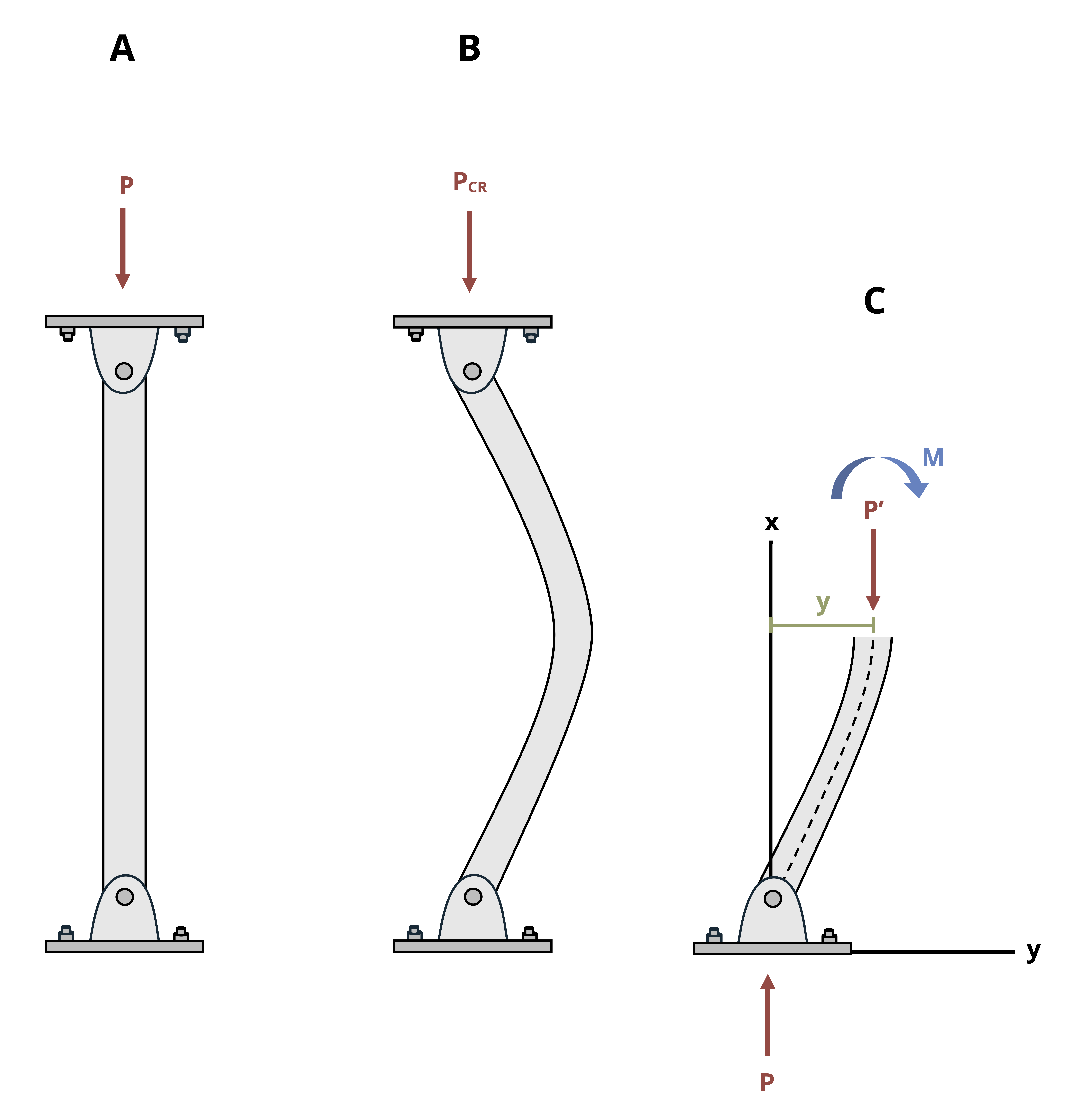
As mentioned in earlier sections, members can fail due to material yielding or fracturing. However, instability represents another critical failure mechanism that requires consideration. Here Euler’s formula can be used to calculate the theoretical buckling load. To do this we’ll start with the simplest of columns, pinned-pinned end connections. This means that the column cannot translate but can rotate as shown in Figure 15.4.
Columns are similar to beams rotated 90°, so we can use what we already know about the elastic curve.
\[ \frac{d^2 y}{d x^2}=\frac{M}{E I} \]
We can use the FBD in Figure 15.4 (C) to sum moments about any point on the lower column section.
\[ \begin{aligned} & \sum M=0=M+P y \\ & M=-P y \end{aligned} \]
We can now substitute this expression into the elastic curve equation.
\[ \begin{aligned} & \frac{d^2 y}{d x^2}=\frac{-P y}{E I} \\ & \frac{d^2 y}{d x^2}+\left(\frac{P}{E I}\right) y=0 \end{aligned} \]
This is a linear, homogeneous, second-order differential equation with constant coefficients, which has a general solution of
\[ y=C_1 \sin \left(\sqrt{\frac{P}{E I}} x\right)+C_2 \cos \left(\sqrt{\frac{P}{E I}} x\right) \]
The two constants, C1 and C2, can be determined by imploring boundary conditions. Since y = 0 at x = 0 and y = 0 when x = L, the first condition results in
\[ \begin{aligned} &0 =C_1(0)+C_2(1) \\ & C_2 =0 \end{aligned} \]
The second boundary condition, x = L when y = 0, results in
\[ 0=C_1 \sin \left(\sqrt{\frac{P}{E I}} x\right)+0 \]
The equation is satisfied if C1 = 0. However, this is a trivial solution that implies y = 0 and there is no lateral deflection. For the nontrivial solution, the sine function must be equal to zero, which requires
\[ \begin{aligned} &\sqrt{\frac{P}{E I}} L=n \pi \\ & \text {where } n=1, 2, 3, 4,... \end{aligned} \]
The smallest value of P occurs when n = 1; substituting this and rearranging gives us Euler’s formula
\[ \boxed{P_{c r}=\frac{\pi^2 E I}{L^2}}\text{ ,} \tag{15.1}\]
Pcr = Critical axial load on the column just before it buckles [N, lb]. (This load must be less than the load that would cause the stress in the column to exceed the yield stress; otherwise due to yield stress the column will fail before it buckles.)
E = Elastic modulus of the material [Pa, psi]
I = Second moment of area for the column [m4, in.4]. (If Ix and Iy differ, use the smaller value.)
L = Unsupported length of the column (pinned-pinned connection) [m, in.]
This formula is named after the Swiss mathematician, Leonhard Euler, who developed it in 1744. Other buckling modes can exist (n = 2, n = 3, n = 4, etc.) but are less commonly used because the load required for the higher modes would be large. The first three buckling loads can be seen in Figure 15.5.
15.1.3 Buckling Direction
Columns pinned at both ends with circular or square cross-sections (equal second moments of area) can buckle in any direction. For columns with asymmetric cross-sections, buckling occurs in the plane perpendicular to the axis with the smallest second moment of area. For example, a ruler in Figure 15.2 with a rectangular cross-section buckles about its weaker axis under compression. For nonsymmetric sections, both axes should be analyzed to find the smallest second moment of area, which is then used to calculate the critical buckling load. Figure 15.6 shows buckling in wood supports.
15.1.4 Critical Stress
The Euler buckling equation can be used to calculate the critical stress for a column by setting I = Ar2, where A is the cross-sectional area and r is the radius of gyration. For a more comprehensive discussion on the radius of gyration, see the Engineering Statics book by Baker and Haynes.
\[ \sigma_{c r}=\frac{P_{c r}}{A}=\frac{\pi^2 E\left(A r^2\right)}{A L^2} \]
Rearranging produces
\[ \boxed{\sigma_{c r}=\frac{\pi^2 E}{\left(\frac{L}{r}\right)^2}}\text{ ,} \tag{15.2}\]
σcr = Critical stress on the column just before it buckles [Pa, psi]. (This stress must be less than that of the yield stress; otherwise due to yield stress the column will fail before it buckles.)
E = Elastic modulus of the material [Pa, psi]
L = Unsupported length of the column (pinned-pinned connection) [m, in.]
r = Smallest radius of gyration of the column [m, in.]
The quantity in the denominator, L/r, is called the slenderness ratio of the column. Many times this ratio is used to classify columns as short, intermediate, or long. The smallest value of the radius of gyration is used to find the critical stress.
A plot of the critical stress versus the slenderness ratio is shown in Figure 15.7. For larger slenderness ratios the curve is hyperbolic. For smaller slenderness ratios the critical stress is equal to the material’s yield stress. This graph illustrates that if the critical stress calculated using Euler’s equation is greater than the yield stress, the stress is of no interest because the column will yield before it has the chance to buckle.
Example 15.1 demonstrates calculation of the critical buckling load and critical buckling stress.
Example 15.1
A pinned-pinned W10 x 30 column is 8 ft long and made of A492 steel (σy = 50 ksi and E = 29,000 ksi).
What is the largest axial load this column can support?
First consult the table in Appendix A to get the section properties of a W10 x 30 section.
\[ \begin{aligned} & A=8.84{~in.}^2 \\ & I_x=170{~in.}^4 \\ & r_y=4.38{~in.} \\ & I_y=16.7{~in.}^4 \\ & r_y=1.37{~in.} \end{aligned} \]
Then start by calculating the critical load using Euler’s buckling formula. Note that we can confidently say that this column will buckle about the y-axis since the second moment of area in the y direction is the smallest.
\[ \begin{aligned} & P_{cr}=\frac{\pi^2 E I}{L^2}=\frac{\pi^2(29,000{~ksi})(16.7{~in.}^4)}{\left(8{~ft}* 12\frac{in.}{ft}\right)^2} \\ & P_{cr}=518.6{~kips} \end{aligned} \]
This represents the load at which any increase in applied load will cause the column to buckle.
Next calculate the stress associated with this critical load.
\[ \sigma_{c r}=\frac{P_{cr}}{A}=\frac{518.6{~kips}}{8.84{~in.^2}}=58.7{~ksi} \]
Since this stress is larger than the yield stress of the steel (σy = 50 ksi), the column will not buckle first. It will fail due to yielding.
Calculate the force using the stress of an axial member formula discussed in Chapter 2.
\[ \begin{aligned} &\sigma_{cr} =\frac{P}{A} \\ & 50{~ksi} =\frac{P}{8.84{~in.}^2} \\ &p =442{~kips} \end{aligned} \]
15.2 Effect of Supports
Click to expand
We derived Euler’s equation for buckling with pinned-pinned supports (the simplest case). However, in many cases columns are supported by other end conditions. Just as Euler’s formula for buckling was derived by solving a differential equation for the pinned-pinned conditions, the same can be done for other types of support cases. We will derive one more here.
Let’s consider the case where a column is fixed at one end and free at the other end as shown in Figure 15.8 (A). Summing moments at the cut end of the FBD in Figure 15.8 (B) yields M = P(δ-y).
We can now write the differential equation using the elastic curve equation.
\[ \begin{aligned} & E I \frac{d^2 y}{d x^2}=P(\delta-y) \\ & \frac{d^2 y}{d x^2}+\left(\frac{P}{E I}\right) y=\left(\frac{P}{E I}\right) \delta \end{aligned} \]
Since the right side is not equal to zero, this equation is nonhomogeneous (note this differs from the earlier derivation for the pinned-pinned connection). There will be a particular and complementary solution.
\[ y=C_1 \sin \left(\sqrt{\frac{P}{E I} x}\right)+C_2 \cos \left(\sqrt{\frac{P}{E I} x}\right)+\delta \]
We can now employ boundary conditions to solve for the constants. At x = 0, y = 0, so C2 = δ. Also at x = 0, dy/dx = 0, so C1 = 0. This leads us to the following deflection curve:
\[ y=\delta\left(1-\cos \left(\sqrt{\frac{P}{E I}} x\right)\right) \]
At the free end of the column, x = L, we know that y = δ, and therefore
\[ 0=\delta \cos \left(\sqrt{\frac{P}{E I} L}\right) \]
The trivial solution δ = 0 shows that no matter what the P value, no buckling will occur. Thus
\[ \begin{aligned} & 0=\cos \left(\sqrt{\frac{P}{E I} L}\right) \\ & \sqrt{\frac{P}{E I}} L=\frac{n \pi}{2} \\ & \text{where n=1, 3, 5,...} \end{aligned} \]
The smallest critical load happens at n = 1 and results in
\[ P_{c r}=\frac{\pi^2 E I}{(2 L)^2} \]
Other support conditions can be derived in a similar manner.
15.2.1 Effective Length
The critical load equation for a fixed-free column differs from a pinned-pinned column only by multiplying the length L by 2. The effective length, Le, is the distance between points where the moment is zero. For a pinned-pinned column, L = Le, as illustrated in Figure 15.9, whereas for a fixed-free column, Le = 2L.
Other common end conditions also relate L to Le. A general equation applies to any support condition by replacing the effective length with KL, where K is the effective length factor.
\[ \boxed{P_{c r}=\frac{\pi^2 E I}{(K L)^2}} \tag{15.3}\]
and
\[ \boxed{\sigma_{c r}=\frac{\pi^2 E}{\left(\frac{K L}{r}\right)^2}} \tag{15.4}\]
Find the effective length factor, K, below each of the end conditions in Figure 15.9.
Example 15.2 and Example 15.3 demonstrate how to calculate the critical buckling load in columns with various different supports.
Example 15.2
Redo Example 15.1 with a fixed-free column.
Consult the table in Appendix A to find the section properties of a W10 x 30 section.
\[ \begin{aligned} & A=8.84{~in.}^2 \\ & I_x=170{~in.}^4 \\ & r_y=4.38{~in.} \\ & I_y=16.7{~in.}^4 \\ & r_y=1.37{~in.} \end{aligned} \]
Start by calculating the critical load using Euler’s buckling formula. Note that we can confidently say that this column will buckle about the y-axis since the second moment of area in the y-direction is the smallest. Use K = 2 for a fixed-free column.
\[ \begin{aligned} & P_{cr}=\frac{\pi^2 E I}{(k L)^2}=\frac{\pi^2(29,000{~ksi})(16.7{~in.^4})}{\left(2*8{~ft}*12~\frac{in.}{ft}\right)^2} \\ & P_{c r}=129.7{~kips} \\ & \end{aligned} \]
This represents the load at which any increase in applied load will cause the column to buckle.
Calculate the stress associated with this critical load.
\[ \sigma_{c r}=\frac{P_{cr}}{A}=\frac{129.7{~kips}}{8.84{~in.^2}}=14.7{~ksi} \]
Since this stress is smaller than the yield stress of the steel (σy = 50 ksi), the column will buckle first at a critical load of 129.7 kips.
Example 15.3
A W12 x 50 column carries a load of 650 kips.
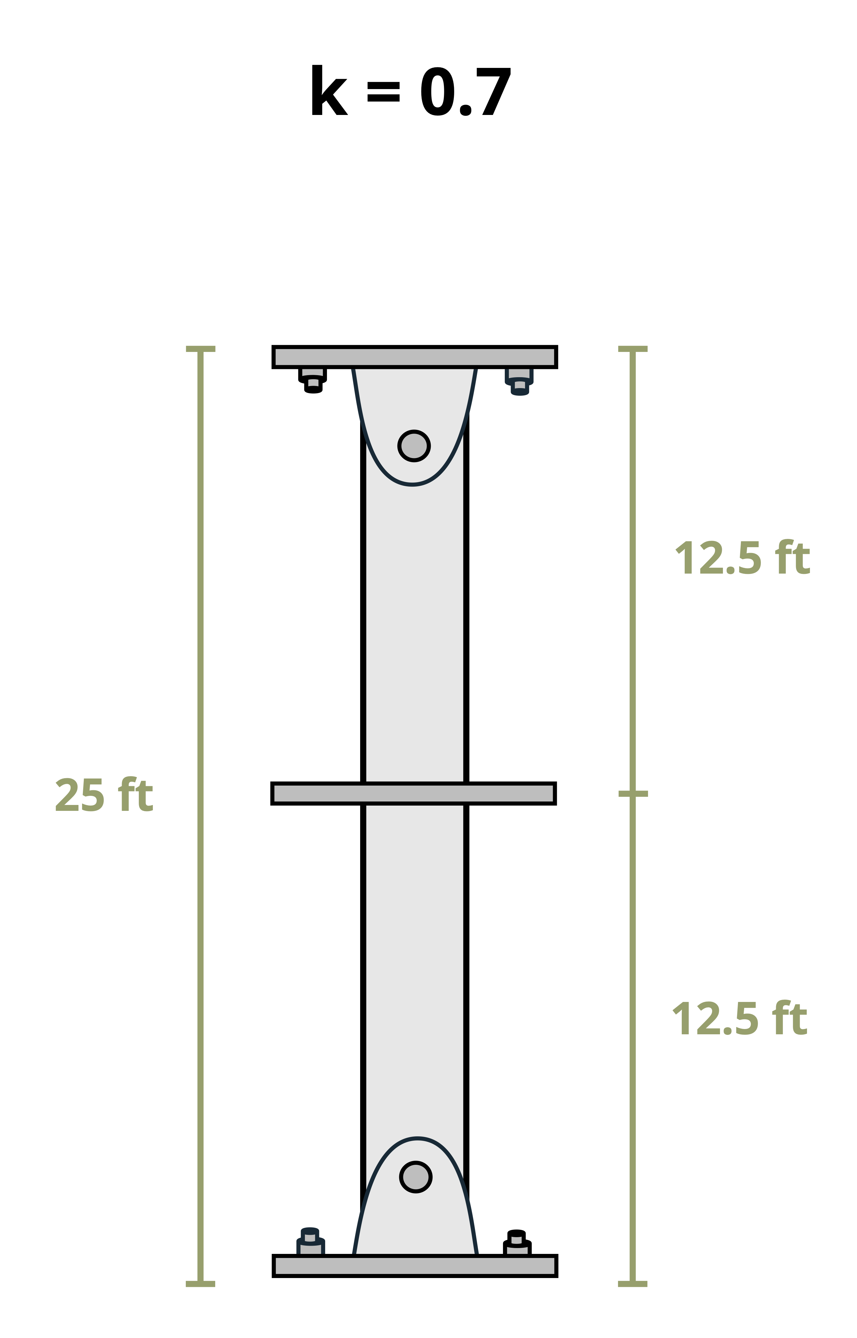
If the column is 25 ft long, has fixed-pinned end conditions, is braced at the midpoint in the weak direction, and is made from A492 steel (σy = 50 ksi and E = 29,000 ksi), is it adequate?
\[ \begin{aligned} & A=14.6{~in.}^2 \\ & I_x=391{~in.}^4 \\ & r_y=5.18{~in.} \\ & I_y=56.3{~in.}^4 \\ & r_y=1.96{~in.} \end{aligned} \]
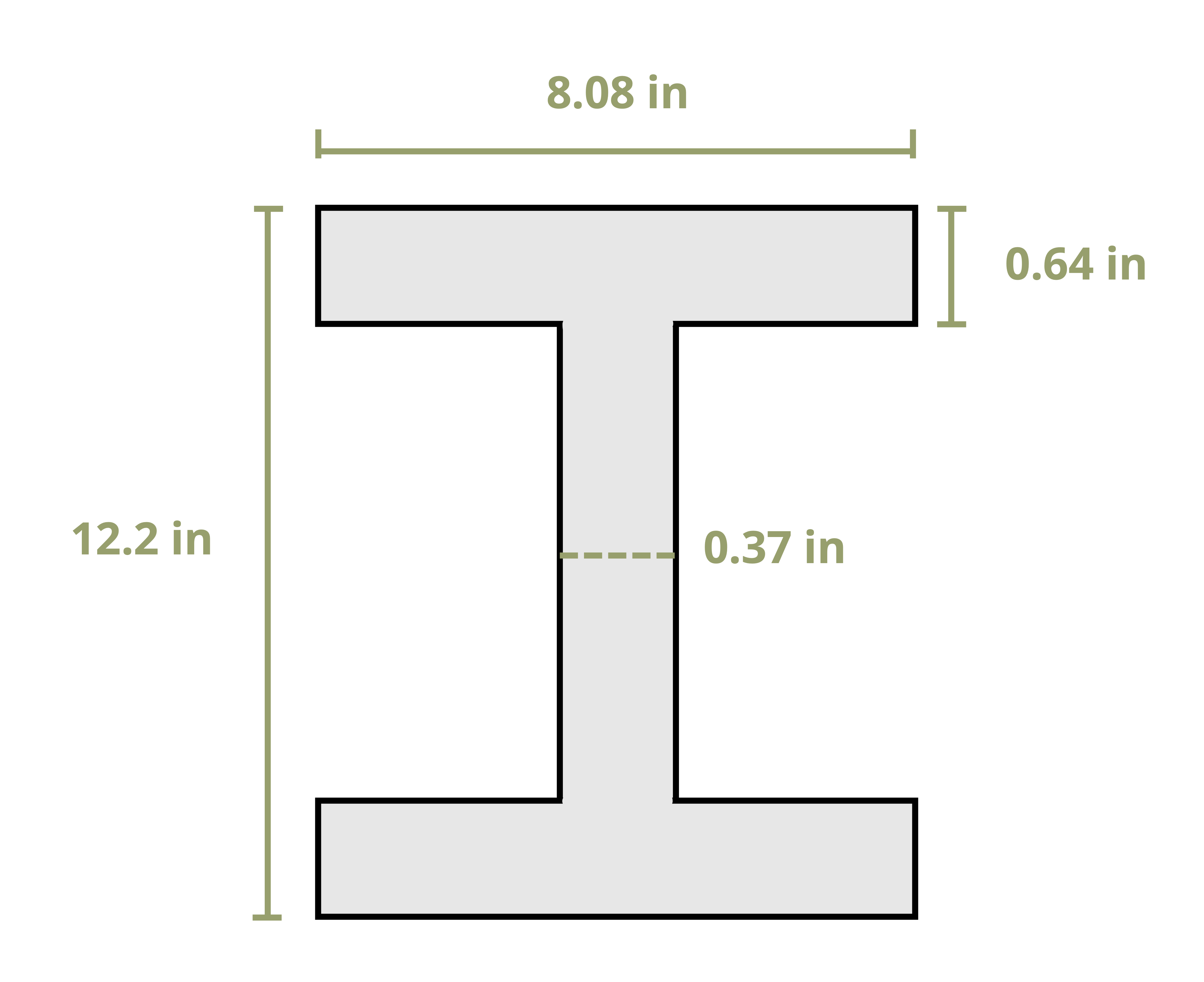
Consult the table in Appendix A to frind the section properties of a W12 x 50 section.
Start by calculating the critical load using Euler’s buckling formula. The brace at the midpoint of the column changes the length of the column in the weak direction. This doesn’t make obvious which axis the column will buckle about, so you need to check both the strong and the weak directions.
Strong axis
\[ \begin{aligned} & P_{cr}=\frac{\pi^2 E I}{(KL)^2}=\frac{\pi^2(29,000{~ksi})(391{~in.}^4)}{\left(0.7*25{~ft}*~12~\frac{in.}{ft}\right)^2} \\ & P_{c r}=2,538{~kips} \\ & \end{aligned} \]
Use the general form of Euler’s buckling equation. Since the end supports are pinned-fixed, use K = 0.7. The critical load in the strong direction is calculated to be 2,538 kips.
Compare this to buckling about the weak axis. The values of I, K, and L will change. The L value changes because the column is braced at the midpoint, so the column has a shorter distance to buckle about. The K value can be tricky, though. There were no details about the brace, so you don’t know if the brace will provide an end condition like a fixed or pinned end. So calculate the worst case, which would be a pinned-pinned end condition (this makes the denominator the largest, so the result will be the smallest).
Weak axis
\[ \begin{aligned} & P_{cr}=\frac{\pi^2 EI}{(KL)^2}=\frac{\pi^2(29,000{~ksi})(56.3{~in.^4})}{\left(1*12.5{~ft}*12\frac{in.}{ft}\right)^2} \\ & P_{c r}=716{~kips} \\ \end{aligned} \]
The critical load in the weak direction is calculated to be 716 kips. This means that if the column were to buckle, it would be about the weak axis since this load was smaller. Because the critical buckling load is greater than the 650 kip applied load, the column is adequate. However, you also need to calculate the load that would cause yielding of the steel.
Yield
\[ \begin{aligned} \sigma_{yield}=\frac{P}{4} \quad\rightarrow\quad &P=(50{~ksi})(14.6{~in.^2}) \\ & P_{yield}=730{~kips} \end{aligned} \]
Given a yielding load of 730 kips, the column is adequate for a 650 kip load. Failure would first occur by buckling in the weak direction if the load were increased to 716 kips. Note that we did not apply any safety factors. In civil engineering, design codes for steel columns designate how to apply safety factors to the loading and the capacity.
What would happen to the capacity of the columns if the brace were not there? To find out, let’s recalculate the critical load for buckling about the weak direction.
No brace
\[ \begin{aligned} & P_{cr}=\frac{\pi^2 E I}{(KL)^2}=\frac{\pi^2(29,000{~ksi})(56.3{in.^4})}{\left(0.7*25{~ft}*12~\frac{in.}{ft}\right)^2} \\ & P_{c r}=365{~kips} \\ \end{aligned} \]
Notice how much lower this is than the braced condition. If the column were not braced, it would be inadequate for the applied load.
Summary
Click to expand
References
Click to expand
Figures
All figures in this chapter were created by Kindred Grey in 2025 and released under a CC BY license, except for
Figure 15.1: Examples of columns. A: Unknown author. 2020. Pixabay license. https://pixabay.com/photos/bridge-tunnel-columns-structure-5441571/. B: ds_30. 2020. Pixabay license. https://pixabay.com/photos/buildings-concrete-construction-4839276/. C: G41rn8. 2009. CC BY-SA. https://commons.wikimedia.org/wiki/File:Hangzhou_2009_1794.jpg.
Figure 15.2: Buckling of a ruler. Amy Richardson. 2024. CC BY-NC-SA.
Figure 15.6: Buckling of wooden studs. scottnj. 2010. CC BY-NC-ND. https://flic.kr/p/8heJAn.